Example
Counterfactual explanations offer an intuitive way to explore how a model’s prediction could change under minimal modifications of the input. Given an instance and a target class, a counterfactual answers the question:
“What is the smallest and most plausible change in this time series that would cause the model to predict a different outcome?”
For multivariate time series, this typically means altering only a short subsequence or specific channels while keeping the overall structure intact. Counterfactuals complement traditional attribution methods by not only highlighting why a decision was made, but also illustrating how it could have been different.
This example walks through the full CONFETTI pipeline for generating such counterfactual explanations, including:
generating a synthetic multivariate time series dataset
training a lightweight FCN classifier
optionally extracting CAM-based feature-importance weights
generating counterfactual candidates
visualizing the resulting explanations
1. Generate a Toy Multivariate Time Series Dataset
We begin by creating a small synthetic dataset with two classes. Each class has a distinct temporal pattern so that a small FCN can achieve reasonable accuracy.
import numpy as np
from pathlib import Path
from confetti.utils import save_multivariate_ts_as_csv

def generate_toy_dataset(
    n_samples=200, timesteps=100, channels=3, random_state=123
):
    rng = np.random.default_rng(random_state)

    X = np.zeros((n_samples, timesteps, channels))
    y = np.zeros(n_samples, dtype=int)

    # Define class patterns
    for i in range(n_samples):
        if i < n_samples // 2:
            # Class 0
            base = np.linspace(0, 2, timesteps)                         # rising trend
            signal = 3.0 * np.sin(np.linspace(0, 3*np.pi, timesteps))   # low freq
            noise = 0.3 * rng.normal(size=(timesteps, channels))
            X[i] = base[:, None] + signal[:, None] + noise
            y[i] = 0
        else:
            # Class 1
            base = np.linspace(2, 0, timesteps)                         # falling trend
            signal = 3.0 * np.sin(np.linspace(0, 12*np.pi, timesteps))  # high freq
            noise = 0.3 * rng.normal(size=(timesteps, channels))
            X[i] = base[:, None] + signal[:, None] + noise
            y[i] = 1

    return X, y


# Create dataset
X, y = generate_toy_dataset()

# Shuffle before split
indices = np.arange(len(X))
np.random.shuffle(indices)
X, y = X[indices], y[indices]

# 80/20 split
split = int(0.8 * len(X))
X_train, y_train = X[:split], y[:split]
X_test, y_test = X[split:], y[split:]

print("Train:", X_train.shape, y_train.shape)
print("Test: ", X_test.shape, y_test.shape)
Train: (160, 100, 3) (160,)
Test:  (40, 100, 3) (40,)
2. Build a Lightweight FCN Classifier
Below is a small FCN-like model designed for example usage.
import keras
from keras import layers
import numpy as np
from pathlib import Path

class ToyFCN:

    def __init__(self, input_shape, num_classes=2):
        self.input_shape   = input_shape
        self.num_classes   = num_classes
        self.model_path    = Path("toy_fcn.keras")
        self.model         = self._build_model()

    def _build_model(self):
        inputs = keras.layers.Input(shape=self.input_shape)

        # Conv block 1
        x = layers.Conv1D(filters=16, kernel_size=8, padding="same")(inputs)
        x = layers.BatchNormalization()(x)
        x = layers.ReLU()(x)

        # Conv block 2
        x = layers.Conv1D(filters=32, kernel_size=5, padding="same")(x)
        x = layers.BatchNormalization()(x)
        x = layers.ReLU()(x)

        # Conv block 3
        x = layers.Conv1D(filters=16, kernel_size=3, padding="same")(x)
        x = layers.BatchNormalization()(x)
        x = layers.ReLU()(x)

        # Global average pooling
        gap = layers.GlobalAveragePooling1D()(x)

        # Output layer
        outputs = layers.Dense(self.num_classes, activation="softmax")(gap)

        model = keras.Model(inputs=inputs, outputs=outputs)
        model.compile(
            optimizer="adam",
            loss="sparse_categorical_crossentropy",
            metrics=["accuracy"],
        )
        return model

    def fit(self, X_train, y_train, epochs=20, batch_size=16, verbose=1):
        self.model.fit(
            X_train,
            y_train,
            epochs=epochs,
            batch_size=batch_size,
            verbose=verbose,
            validation_split=0.2,
        )
        self.model.save(self.model_path)
        return self.model

    def predict(self, X):
        proba = self.model.predict(X)
        return np.argmax(proba, axis=1)

    def predict_proba(self, X):
        return self.model.predict(X)
3. Train the FCN Model
input_shape = X_train.shape[1:]
num_classes = len(np.unique(y_train))

model = ToyFCN(input_shape=input_shape, num_classes=num_classes)

print("Training ToyFCN...")
model.fit(X_train, y_train, epochs=20, batch_size=16, verbose=1)

accuracy = (model.predict(X_test) == y_test).mean()
print(f"Test accuracy: {accuracy:.3f}")
Test accuracy: 1.000
4. Generate Counterfactual Explanations with CONFETTI
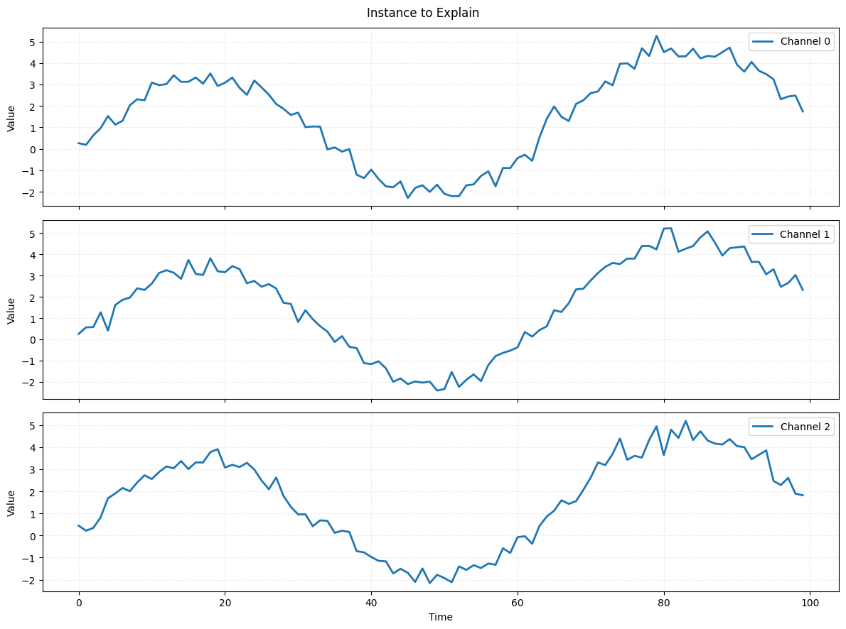
Lets visualize the instance we want to explain.
from confetti.visualizations import plot_time_series

instance = X_test[0:1]
plot_time_series(series=instance, title="Instance to Explain")
Now we apply CONFETTI to generate a counterfactual for a single instance.
from confetti import CONFETTI
from confetti.attribution import cam

weights = cam(model.model, X_train)

instance = X_test[0:1]

explainer = CONFETTI(model_path="toy_fcn.keras")

results = explainer.generate_counterfactuals(
    instances_to_explain=instance,
    reference_data=X_train,
    reference_weights=weights,
    alpha=0.5,
    theta=0.51,
)

cf_set = results[0]
print("Original label:     ", cf_set.original_label)
print("Counterfactual label:", cf_set.best.label)
print("Total generated:     ", len(cf_set.all_counterfactuals))
Original label:      0
Counterfactual label: 1
Total generated:      11
The returned CounterfactualResults object contains several attributes, including the original instance, generated candidates, the best counterfactual, and CAM importance values (when available).
5. Visualize the Counterfactual Explanation
Finally, we visualize the best counterfactual and optional CAM heatmap.
from confetti.visualizations import plot_counterfactual

plot_counterfactual(
    original=cf_set.original_instance,
    counterfactual=cf_set.best,
    cam_weights=cf_set.feature_importance,
    cam_mode="heatmap",
    title="Counterfactual Explanation",
)
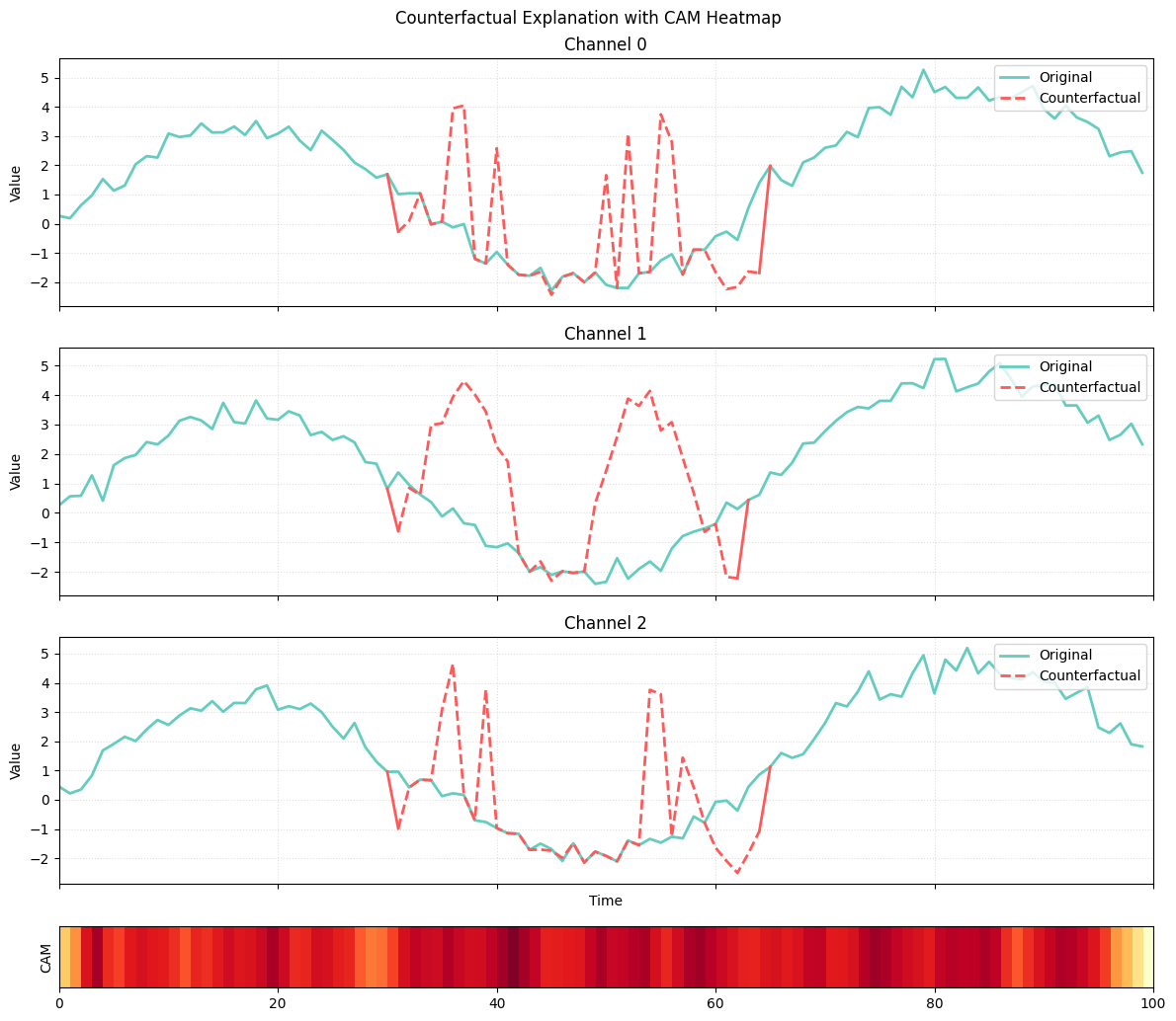
The plot shows how CONFETTI generates a counterfactual by selectively modifying only the most relevant part of the time series. The green curves represent the original instance across all channels, while the red curves show the counterfactual subsequence inserted by the method. The heatmap at the bottom corresponds to the class activation map (CAM) of the nearest unlike neighbor (NUN), which indicates the time region the model relies on most when predicting the new class. CONFETTI uses this CAM as a guide, focusing its perturbation on the segment most responsible for distinguishing the NUN’s class from the original. The alignment between the high-activation region in the CAM and the red counterfactual subsequence illustrates how the method leverages attribution to produce focused and meaningful counterfactual changes.
Alternative: PyTorch Workflow
CONFETTI also supports PyTorch models via
TorchModelAdapter. The sections below mirror
the Keras walkthrough above, reusing the same toy dataset generated in
Section 1.
6a. Build a PyTorch Classifier
The architecture mirrors the Keras ToyFCN: three convolutional
blocks (16 → 32 → 16 filters, kernel sizes 8 → 5 → 3) with batch
normalization and ReLU, followed by global average pooling and a linear
classifier with softmax output.
PyTorch Conv1d expects channels-first input (N, C, T),
whereas CONFETTI stores data as (N, T, C).
TorchModelAdapter handles this permutation
automatically.
import torch
import torch.nn as nn

class ToyFCN(nn.Module):

    def __init__(self, in_channels=3, num_classes=2):
        super().__init__()
        self.conv1 = nn.Conv1d(in_channels, 16, kernel_size=8, padding="same")
        self.bn1 = nn.BatchNorm1d(16)
        self.conv2 = nn.Conv1d(16, 32, kernel_size=5, padding="same")
        self.bn2 = nn.BatchNorm1d(32)
        self.conv3 = nn.Conv1d(32, 16, kernel_size=3, padding="same")
        self.bn3 = nn.BatchNorm1d(16)
        self.classifier = nn.Linear(16, num_classes)

    def forward(self, x):
        x = torch.relu(self.bn1(self.conv1(x)))
        x = torch.relu(self.bn2(self.conv2(x)))
        x = torch.relu(self.bn3(self.conv3(x)))
        x = x.mean(dim=-1)  # global average pooling over time
        x = torch.softmax(self.classifier(x), dim=-1)
        return x
6b. Train and Save
model = ToyFCN(in_channels=3, num_classes=2)
optimizer = torch.optim.Adam(model.parameters(), lr=1e-3)
criterion = nn.CrossEntropyLoss()

# Permute to channels-first for PyTorch
X_train_t = torch.tensor(X_train, dtype=torch.float32).permute(0, 2, 1)
y_train_t = torch.tensor(y_train, dtype=torch.long)

model.train()
for epoch in range(20):
    optimizer.zero_grad()
    logits = model(X_train_t)
    loss = criterion(logits, y_train_t)
    loss.backward()
    optimizer.step()

# Save the full model (not just state_dict)
torch.save(model, "toy_fcn.pt")
Test accuracy: 1.000
Note
torch.save(model, path) serializes the full model object.
CONFETTI’s internal loader (_load_model) uses
torch.load(path, weights_only=False) and wraps the result in a
TorchModelAdapter, so the file must contain the complete
model—not just state_dict.
6c. Wrap with TorchModelAdapter
from confetti import TorchModelAdapter

adapter = TorchModelAdapter(model)
TorchModelAdapter provides a .predict() method that accepts
CONFETTI’s channels-last (N, T, C) arrays and returns class
probabilities as a numpy array. By default channels_last=True, so
the adapter permutes inputs to (N, C, T) before calling the model.
6d. CAM with PyTorch
from confetti.attribution import cam

weights = cam(adapter, X_train)
The cam() function supports both Keras and PyTorch models. In the
Keras example (Section 4), a raw keras.Model was passed; here we
pass the TorchModelAdapter. Internally, CONFETTI uses forward hooks
on Conv1d and Linear layers to capture activations and
classifier weights.
6e. Generate Counterfactuals
from confetti import CONFETTI

explainer = CONFETTI(model_path="toy_fcn.pt")

results = explainer.generate_counterfactuals(
    instances_to_explain=instance,
    reference_data=X_train,
    reference_weights=weights,
    alpha=0.5,
    theta=0.51,
)

cf_set = results[0]
print("Original label:     ", cf_set.original_label)
print("Counterfactual label:", cf_set.best.label)
print("Total generated:     ", len(cf_set.all_counterfactuals))
When CONFETTI receives a .pt or .pth model path it
automatically loads the model with torch.load and wraps it in a
TorchModelAdapter—no manual wrapping is needed for the explainer.
6f. Visualize
from confetti.visualizations import plot_counterfactual

plot_counterfactual(
    original=cf_set.original_instance,
    counterfactual=cf_set.best,
    cam_weights=cf_set.feature_importance,
    cam_mode="heatmap",
    title="Counterfactual Explanation (PyTorch)",
)
The visualization API is identical regardless of framework.